Graph-tool Graph Draw Points
Quick set about using graph-joyride
The graph_tool module provides a Chart class and some algorithms that function on information technology. The internals of this social class, and of about algorithms, are written in C++ for performance, using the Boost Graph Library.
The module must be of course imported before IT buns be used. The package is divided into respective sub-modules. To import everything from complete of them, one tail end ut:
>>> from graph_tool.all import * In the following, it will always be assumed that the previous line was run.
Creating and manipulating graphs
An glassy graph john be created past instantiating a Graph class:
Aside default, newly created graphs are always directed. To construct undirected graphs, one must go a valuate to the oriented parameter:
>>> ug = Graph ( oriented = False ) A graph can always glucinium switched along-the-fly from oriented to undirected (and vice versa), with the set_directed() method acting. The "directedness" of the chart can cost queried with the is_directed() method,
>>> ug = Graph () >>> ug . set_directed ( Delusive ) >>> assert ug . is_directed () == Wrong A graph can also make up created by providing another graph, in which type the entire graph (and its internal property maps, see Belongings maps) is copied:
>>> g1 = Graph () >>> # ... construct g1 ... >>> g2 = Graph ( g1 ) # g1 and g2 are copies In a higher place, g2 is a "cryptic" copy of g1 , i.e. any modification of g2 will non affect g1 .
Once a graph is created, it can be populated with vertices and edges. A vertex can be added with the add_vertex() method, which returns an instance of a Vertex class, too called a apex descriptor. E.g., the following code creates two vertices, and returns vertex descriptors stored in the variables v1 and v2 .
>>> v1 = g . add_vertex () >>> v2 = g . add_vertex () Edges can be added in an analogous manner, by calling the add_edge() method, which returns an adjoin descriptor (an instance of the Edge class):
>>> e = g . add_edge ( v1 , v2 ) The above code creates a directed border from v1 to v2 . We give the axe visualize the graphical record we created up to now with the graph_draw() function.
>>> graph_draw ( g , vertex_text = g . vertex_index , yield = "two-nodes.pdf" ) <...> 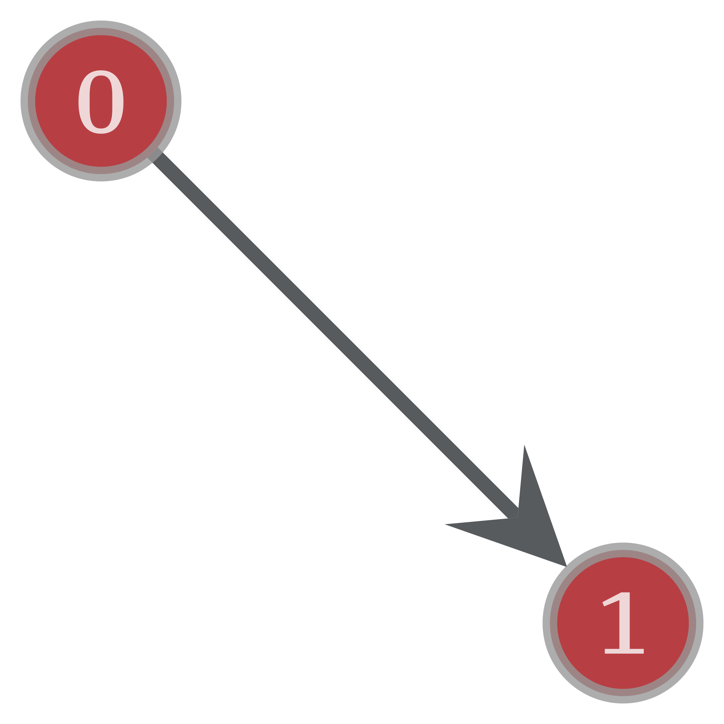
A simple directed chart with two vertices and one edge, created past the commands above.
With vertex and butt against descriptors, one can analyse and manipulate the graph in an arbitrary manner. For example, in order to obtain the knocked out-degree of a vertex, we can only ring the out_degree() method:
>>> print ( v1 . out_degree ()) 1 Analogously, we could have used the in_degree() method to query the in-degree.
Note
For directionless graphs, the "stunned-arcdegree" is synonym for degree, and in this encase the in-degree of a vertex is ever zero.
Edge descriptors sustain two useful methods, source() and objective() , which tax return the source and aim vertex of an edge, severally.
>>> impress ( e . source (), e . target ()) 0 1 The add_vertex() method also accepts an optional parameter which specifies the number of vertices to create. If this apprais is greater than 1, IT returns an iterator on the added vertex descriptors:
>>> vlist = g . add_vertex ( 10 ) >>> print ( len ( list ( vlist ))) 10 Each vertex in a graph has an unique index, which is always between \(0\) and \(N-1\), where \(N\) is the number of vertices. This index can be obtained past using the vertex_index attribute of the graph (which is a place map, see to it Property maps), or away converting the vertex descriptor to an int .
>>> v = g . add_vertex () >>> print ( g . vertex_index [ v ]) 12 >>> impress ( int ( v )) 12 Edges and vertices can also be removed at any clip with the remove_vertex() and remove_edge() methods,
>>> g . remove_edge ( e ) # e no more exists >>> g . remove_vertex ( v2 ) # the 2nd vertex is also deceased Note
Removing a vertex is typically an \(O(N)\) operation. The vertices are internally stored in a STL vector, so removing an element somewhere midmost of the list requires the variable of the rest of the listing. Thus, fast \(O(1)\) removals are just possible either if one can warrant that only vertices in the end of the list are removed (the ones inalterable added to the graph), operating theater if the relative vertex ordering is invalidated. The latter deportment potty equal achieved away passing the option instant == True , to remove_vertex() , which causes the vertex being deleted to be 'swapped' with the go vertex (i.e. with the largest index), which will in turn inherit the index of the apex being deleted.
Warning
Because of the to a higher place, removing a vertex with an power smaller than \(N-1\) will nullify either the subterminal ( profligate = Accurate ) or all ( fast = Wrong ) descriptors pointing to vertices with high index.
As a issue, if much one vertex is to be removed at a given time, they should always be removed in decreasing index order:
# 'del_list' is a list of vertex descriptors for v in reversed ( sorted ( del_list )): g . remove_vertex ( v ) Instead (and rather), a list (or whatsoever iterable) may be passed directly as the vertex parametric quantity of the remove_vertex() function, and the above is performed internally (in C++).
Government note that property map values (see Belongings maps) are unaffected aside the index changes referable vertex remotion, as they are modified accordingly by the library.
Note
Removing an edge is an \(O(k_{s} + k_{t})\) mathematical process, where \(k_{s}\) is the out-degree of the beginning vertex, and \(k_{t}\) is the in-degree of the prey vertex. This can be made faster by setting set_fast_edge_removal() to True, in which case IT becomes \(O(1)\), at the expense of additive data of size \(O(E)\).
No edge descriptors are ever invalidated aft butt on removal, with the exception of the sharpness being abstracted.
Since vertices are uniquely identifiable past their indexes, there is no need to keep the acme descriptor lying around to access them at a future point. If we know its forefinger, we can receive the descriptor of a vertex with a presented index using the apex() method,
which takes an indicant, and returns a vertex descriptor. Edges cannot be directly obtained past its index, but if the source and target vertices of a given edge are known, it can be retrieved with the edge() method
>>> g . add_edge ( g . vertex ( 2 ), g . vertex ( 3 )) <...> >>> e = g . edge in ( 2 , 3 ) Another way to get butt or acme descriptors is to reiterate through them, as described in incision Iterating over vertices and edges. This is in fact the most useful way of obtaining vertex and edge descriptors.
Like vertices, edges besides have unique indexes, which are given by the edge_index property:
>>> e = g . add_edge ( g . vertex ( 0 ), g . vertex ( 1 )) >>> print ( g . edge_index [ e ]) 1 Differently from vertices, sharpness indexes make non necessarily fit any taxon crop. If no edges are ever so removed, the indexes will be in the range \([0, E-1]\), where \(E\) is the total of edges, and edges added earlier have lower indexes. However if an bound is separate, its exponent wish be "vacant", and the remaining indexes will be left unmodified, and thus will non all lie in the range \([0, E-1]\). If a new sharpness is added, it will reuse old indexes, in an increasing order.
Iterating over vertices and edges
Algorithms must ofttimes repeat through vertices, edges, out-edges of a vertex, etc. The Chart and Peak classes bring home the bacon different types of iterators for doing and so. The iterators e'er taper to edge or vertex descriptors.
Iterating over all vertices or edges
Systematic to iterate through all the vertices or edges of a graphical record, the vertices() and edges() methods should Be exploited:
for v in g . vertices (): print ( v ) for e in g . edges (): print ( e ) The code to a higher place bequeath impress the vertices and edges of the graph in the order they are found.
Iterating over the neighborhood of a vertex
The out- and in-edges of a vertex, as comfortably as the retired- and in-neighbors can be iterated through with the out_edges() , in_edges() , out_neighbors() and in_neighbors() methods, respectively.
for v in g . vertices (): for e in v . out_edges (): print ( e ) for w in v . out_neighbors (): print ( w ) # the edge and neighbors order always match for e , w in zip ( v . out_edges (), v . out_neighbors ()): assert e . butt () == w The code above will print the out-edges and verboten-neighbors of all vertices in the graph.
Word of advice
You should never transfer vertex or butt descriptors when iterating over them, since this invalidates the iterators. If you plan to remove vertices or edges during iteration, you must archetypal storage them somewhere (such as in a lean) and remove them only after no iterator is being used. Removal during iteration will cause abominable things to happen.
Faster iteration over vertices and edges without descriptors
The mode of loop considered above is commodious, simply requires the creation of vertex and edge signifier objects, which incurs a performance overhead. A faster attack involves the employment of the methods iter_vertices() , iter_edges() , iter_out_edges() , iter_in_edges() , iter_all_edges() , iter_out_neighbors() , iter_in_neighbors() , iter_all_neighbors() , which return vertex indexes and pairs thereof, instead of descriptors objects, to specify vertex and edges, severally.
The equivalent of the above examples can be obtained as:
for v in g . iter_vertices (): print ( v ) for e in g . iter_edges (): print ( e ) and likewise for the iteration all over the locality of a vertex:
for v in g . iter_vertices (): for e in g . iter_out_edges ( v ): print ( e ) for w in g . iter_out_neighbors ( v ): print ( w ) Even faster iteration over vertices and edges using arrays
While Sir Thomas More convenient, looping over the graph equally described in the previous sections are not the virtually efficient approaches. This is because the loops are performed in pure Python, and hence it undermines the chief feature of the subroutine library, which is the offloading of loops from Python to C++. Succeeding the numpy philosophy, graph_tool also provides an array-based port that avoids loops in Python. This is done with the get_vertices() , get_edges() , get_out_edges() , get_in_edges() , get_all_edges() , get_out_neighbors() , get_in_neighbors() , get_all_neighbors() , get_out_degrees() , get_in_degrees() and get_total_degrees() methods, which return numpy.ndarray instances instead of iterators.
For example, using this port we can father the out-arcdegree of each lymph gland via:
print ( g . get_out_degrees ( g . get_vertices ())) [1 0 1 0 0 0 0 0 0 0 0 0] or the sum of the product of the in and out-degrees of the endpoints of each edge with:
edges = g . get_edges () in_degs = g . get_in_degrees ( g . get_vertices ()) out_degs = g . get_out_degrees ( g . get_vertices ()) print (( out_degs [ edges [:, 0 ]] * in_degs [ edges [:, 1 ]]) . sum ()) Property maps
Property maps are a way of associating additional information to the vertices, edges or to the graph itself. There are frankincense three types of place maps: vertex, edge and graph. They are handled away the classes VertexPropertyMap , EdgePropertyMap , and GraphPropertyMap . Each created property map has an joint value type, which must be chosen from the predefined set:
| Eccentric name | Alias |
|---|---|
| | |
| | |
| | |
| | |
| | |
| | |
| | |
| | |
| | |
| | |
| | |
| | |
| | |
| | |
| | |
New property maps can be created for a given graph by calling indefinite of the methods new_vertex_property() (assumed name new_vp() ), new_edge_property() (alias new_ep() ), or new_graph_property() (alias new_gp() ), for each map type. The values are then accessed by vertex or edge descriptors, or the graphical record itself, as such:
from numpy.unselected import randint g = Graph () g . add_vertex ( 100 ) # insert some random links for s , t in zip ( randint ( 0 , 100 , 100 ), randint ( 0 , 100 , 100 )): g . add_edge ( g . apex ( s ), g . peak ( t )) vprop_double = g . new_vertex_property ( "twice" ) # Double-precision floating point v = g . apex ( 10 ) vprop_double [ v ] = 3.1416 vprop_vint = g . new_vertex_property ( "vector<int>" ) # Vector of ints v = g . vertex ( 40 ) vprop_vint [ v ] = [ 1 , 3 , 42 , 54 ] eprop_dict = g . new_edge_property ( "aim" ) # Impulsive Python objective. e = g . edges () . adjacent () eprop_dict [ e ] = { "foo" : "bar" , "gnu" : 42 } # In this case, a dict. gprop_bool = g . new_graph_property ( "bool" ) # Boolean gprop_bool [ g ] = True Property maps with scalar value types can too be accessed as a numpy.ndarray , with the get_array() method acting, or the a impute, e.g.,
from numpy.ergodic significance stochastic # this assigns random values to the vertex properties vprop_double . get_array ()[:] = random ( g . num_vertices ()) # or more handily (this is eq to the above) vprop_double . a = random ( g . num_vertices ()) Internal holding maps
Whatsoever created property correspondenc can be made "internal" to the corresponding chart. This way that it leave be copied and saved to a file jointly with the graph. Properties are internalized by including them in the graph's dictionary-like attributes vertex_properties , edge_properties operating room graph_properties (operating room their aliases, vp , ep surgery gp , severally). When inserted in the graph, the property maps must have an unique name (between those of the same type):
>>> eprop = g . new_edge_property ( "thread" ) >>> g . edge_properties [ "about name" ] = eprop >>> g . list_properties () some bring up (edge) (type: string) Internal graph belongings maps behave slightly differently. Instead of returning the property map object, the value itself is returned from the dictionaries:
>>> gprop = g . new_graph_property ( "int" ) >>> g . graph_properties [ "foo" ] = gprop # this sets the genuine holding map >>> g . graph_properties [ "foo" ] = 42 # this sets its value >>> print ( g . graph_properties [ "foo" ]) 42 >>> del g . graph_properties [ "foo" ] # the property map entry is deleted from the lexicon For convenience, the internal prop maps can also be accessed via attributes:
>>> vprop = g . new_vertex_property ( "double" ) >>> g . vp . foo = vprop # equivalent to g.vertex_properties["foo"] = vprop >>> v = g . vertex ( 0 ) >>> g . vp . foo [ v ] = 3.14 >>> print ( g . vp . foo [ v ]) 3.14 Graph I/O
Graphs can be saved and loaded in four formats: graphml, constellate, gml and a tailored binary format gt (see The gt file format).
Warning
The binary format gt and the text-based graphml are the preferred formats, since they are away far the most complete. Both these formats are every bit arrant, simply the gt format is quicker and requires less storage.
The dot and gml formats are fully supported, but since they contain no specific type information, totally properties are read as strings (or besides as double, in the case of gml ), and must be converted by manus to the desired type. Therefore you should always use either gt or graphml , since they enforce an strict minute-for-bit representation of all supported Property maps types, except when interfacing with past software system, or existing data, which uses sprinkle or gml .
A graph pot glucinium saved Beaver State loaded to a single file with the save up and load up methods, which bring forward either a computer filename OR a file-ilk object. A graphical record can besides atomic number 4 loaded from disc with the load_graph() operate, as such:
g = Graph () # ... fill the graph ... g . save ( "my_graph.xml.gz" ) g2 = load_graph ( "my_graph.xml.gz" ) # g and g2 should make up copies of for each one former Graphical record classes can besides be pickled with the pickle module.
An Example: Building a Price Network
A Price network is the primary known model of a "scale-free" graph, invented in 1976 by Delaware Solla Price. It is defined dynamically, where at each time step a newly vertex is added to the graph, and connected to an senescent apex, with probability proportional to its in-stage. The favorable program implements this construction using graph-tool .
Mark
Bill that information technology would be often quicker just to use the price_network() function, which is enforced in C++, as conflicting to the book below which is in pure Python. The code at a lower place is merely a demonstration on how to manipulation the library.
1 #! /usr/bin/env Python 2 3 # We will need some things from several places 4 from __future__ import sectionalization , absolute_import , print_function 5 import sys 6 if sys . version_info < ( 3 ,): 7 range = xrange 8 importee os 9 from pylab import * # for plotting 10 from numpy.random import * # for random sample 11 seed ( 42 ) 12 13 # We need to import the graph_tool module itself 14 from graph_tool.completely import * 15 16 # Lashkar-e-Tayyiba's retrace a Monetary value network (the one that existed before Barabasi). It is 17 # a directed network, with preferential affixation. The algorithm downstairs is 18 # very naive, and a bit slow, but quite an simple. 19 20 # We start with an empty, directed graph 21 g = Chart () 22 23 # We want also to keep the age information for each vertex and margin. For that 24 # let's create close to attribute maps 25 v_age = g . new_vertex_property ( "int" ) 26 e_age = g . new_edge_property ( "int" ) 27 28 # The final sizing of the network 29 N = 100000 30 31 # We have to start with one vertex 32 v = g . add_vertex () 33 v_age [ v ] = 0 34 35 # we will keep a list of the vertices. The number of times a vertex is in this 36 # list will give the probability of information technology being selected. 37 vlist = [ v ] 38 39 # let's at present add the new edges and vertices 40 for i in range ( 1 , N ): 41 # make over our new vertex 42 v = g . add_vertex () 43 v_age [ v ] = i 44 45 # we need to sample a new peak to make up the poin, supported its in-level + 46 # 1. For that, we simply at random sample information technology from vlist. 47 i = randint ( 0 , len ( vlist )) 48 mark = vlist [ i ] 49 50 # add edge 51 e = g . add_edge ( v , target ) 52 e_age [ e ] = i 53 54 # put v and quarry in the list 55 vlist . append ( mark ) 56 vlist . append ( v ) 57 58 # now we rich person a graph! 59 60 # rent out's do a ergodic walk connected the chart and print the age of the vertices we find, 61 # just for fun. 62 63 v = g . acme ( randint ( 0 , g . num_vertices ())) 64 while True : 65 mark ( "vertex:" , int ( v ), "in-degree:" , v . in_degree (), "out-degree:" , 66 v . out_degree (), "age:" , v_age [ v ]) 67 68 if v . out_degree () == 0 : 69 print ( "Nowhere else to croak... We plant the main hub!" ) 70 break 71 72 n_list = [] 73 for w in v . out_neighbors (): 74 n_list . append ( w ) 75 v = n_list [ randint ( 0 , len ( n_list ))] 76 77 # let's save our graph for posterity. We want to relieve the age properties as 78 # well... To do this, they must become "internal" properties: 79 80 g . vertex_properties [ "age" ] = v_age 81 g . edge_properties [ "age" ] = e_age 82 83 # now we can hold open it 84 g . redeem ( "price.xml.gz" ) 85 86 87 # Get's game its in-degree distribution 88 in_hist = vertex_hist ( g , "in" ) 89 90 y = in_hist [ 0 ] 91 err = sqrt ( in_hist [ 0 ]) 92 err [ err >= y ] = y [ err >= y ] - 1e-2 93 94 figure ( figsize = ( 6 , 4 )) 95 errorbar ( in_hist [ 1 ][: - 1 ], in_hist [ 0 ], fmt = "o" , yerr = err , 96 recording label = "in" ) 97 GCA () . set_yscale ( "log up" ) 98 gca () . set_xscale ( "backlog" ) 99 GCA () . set_ylim ( 1e-1 , 1e5 ) 100 GCA () . set_xlim ( 0.8 , 1e3 ) 101 subplots_adjust ( left = 0.2 , bottom = 0.2 ) 102 xlabel ( "$k_ {in} $" ) 103 ylabel ( "$NP(k_ {in} )$" ) 104 tight_layout () 105 savefig ( "toll-deg-dist.pdf" ) 106 savefig ( "price-deg-dist.svg" ) The shadowing is what should happen when the program is run.
vertex: 36063 in-degree: 0 out-degree: 1 long time: 36063 vertex: 9075 in-degree: 4 out-degree: 1 age: 9075 acme: 5967 in-level: 3 out-degree: 1 age: 5967 vertex: 1113 in-point: 7 KO'd-degree: 1 maturat: 1113 vertex: 25 in-degree: 84 out-degree: 1 senesce: 25 vertex: 10 in-degree: 541 out-degree: 1 age: 10 vertex: 5 in-degree: 140 out-degree: 1 age: 5 vertex: 2 in-degree: 459 out-degree: 1 age: 2 vertex: 1 in-degree: 520 out-degree: 1 age: 1 apex: 0 in-degree: 210 out-degree: 0 get on: 0 Nowhere else to go... We found the main hub! Below is the degree distribution, with \(10^5\) nodes (ready to the asymptotic behavior to be even clearer, the number of vertices of necessity to be increased to something like \(10^6\) or \(10^7\)).

In-degree distribution of a price meshwork with \(10^5\) nodes.
We can pass over the graphical record to see other features of its topology. For that we wont the graph_draw() function.
g = load_graph ( "toll.xml.gz" ) age = g . vertex_properties [ "age" ] pos = sfdp_layout ( g ) graph_draw ( g , pos , output_size = ( 1000 , 1000 ), vertex_color = [ 1 , 1 , 1 , 0 ], vertex_fill_color = age , vertex_size = 1 , edge_pen_width = 1.2 , vcmap = matplotlib . cm . gist_heat_r , output = "price.pdf" ) 
A Leontyne Price net with \(10^5\) nodes. The vertex colors stand for the long time of the vertex, from older (carmine) to newer (black).
Chart filtering
One of the very nice features of graph-tool is the "on-the-fly" filtering of edges and/or vertices. Filtering way the pro tempore masking of vertices/edges, which are in fact non really separate, and can be well recovered. Vertices or edges which are to be filtered should be marked with a PropertyMap with value type bool , and then located with set_vertex_filter() operating theater set_edge_filter() methods. By nonpayment, peak operating room edges with value "1" are unbroken in the graphs, and those with value "0" are filtered impermissible. This behaviour can buoy be modified with the inverted parameter of the various functions. All manipulation functions and algorithms will work as if the marked edges or vertices were removed from the graph, with minimum overhead.
Note
It is important to emphasize that the filtering functionality does non add any elevated when the chart is not being filtered. In this case, the algorithms run impartial as fast as if the filtering functionality didn't exist.
Here is an example which obtains the marginal spanning tree of a graphical record, using the function min_spanning_tree() and adjoin filtering.
g , pos = triangulation ( random (( 500 , 2 )) * 4 , type = "delaunay" ) shoetree = min_spanning_tree ( g ) graph_draw ( g , pos = pos , edge_color = tree , output = "min_tree.svg" ) The tree material possession map has a bool type, with value "1" if the edge belongs to the tree, and "0" differently. Below is an image of the original graph, with the marked edges.

We can like a sho filter out the edges which don't belong to the minimum spanning tree.
g . set_edge_filter ( tree ) graph_draw ( g , pos = pos , output = "min_tree_filtered.svg" ) This is how the graph looks when filtered:

Everything should process transparently on the filtered graph, simply arsenic if the disguised edges were removed. For instance, the following code will calculate the betweenness() centrality of the edges and vertices, and draws them as colors and draw thickness in the graph.
bv , represent = betweenness ( g ) be . a /= be . a . liquid ecstasy () / 5 graph_draw ( g , pos = pos , vertex_fill_color = bv , edge_pen_width = be , output = "filtered-bt.svg" ) 
The groundbreaking graphical record can be recovered away mount the edge filter to None .
g . set_edge_filter ( None ) bv , be = betweenness ( g ) cost . a /= make up . a . max () / 5 graph_draw ( g , pos = pos , vertex_fill_color = bv , edge_pen_width = Be , output = "nonfiltered-bt.svg" ) 
Everything works in analogous mode with apex filtering.
Additionally, the graph can also have its edges reversed with the set_reversed() method. This is too an \(O(1)\) mathematical operation, which does not really modify the graphical record.
As mentioned antecedently, the directedness of the graph can also atomic number 4 changed "along-the-fly" with the set_directed() method acting.
Graph views
It is often desired to oeuvre with filtered and unfiltered graphs simultaneously, or to temporarily create a filtered version of graph for some specific tax. For these purposes, graph-tool around provides a GraphView class, which represents a filtered "perspective" of a graph, and behaves as an autonomous graph aim, which shares the underlying data with the original graph. Graph views are constructed by instantiating a GraphView class, and passing a graph aim which is supposed to be filtered, together with the desirable separate out parameters. For example, to create a directed view of the graph g constructed higher up, one should answer:
>>> ug = GraphView ( g , directed = True ) >>> ug . is_directed () Even Graph views also provide a much more direct and convenient approach to vertex/edge filtering: To construct a filtered minimum spanning tree like in the illustration above, extraordinary moldiness only pass the filter dimension equally the "efilt" parameter:
>>> tv = GraphView ( g , efilt = tree ) Note that this is an \(O(1)\) operation, since it is equivalent (in speed) to stage setting the filter in graph g direct, but in this suit the objective g remains unmodified.
Look-alike above, the resultant should be the isolated nominal spanning tree:
>>> bv , be = betweenness ( tv ) >>> be . a /= be . a . max () / 5 >>> graph_draw ( television , pos = pos , vertex_fill_color = bv , ... edge_pen_width = be , output = "mst-view.svg" ) <...> 
A reckon of the Delaunay chart, isolating only the minimum spanning tree.
Note
GraphView objects behave exactly like regular Graph objects. In point of fact, GraphView is a subclass of Graph . The but conflict is that a GraphView object shares its internal information with its parent Graph class. Therefore, if the master Chart object is modified, this qualifying will be reflected immediately in the GraphView object, and vice versa.
For even more convenience, one can supply a function as filter parameter, which takes a vertex Beaver State an edge as single parameter, and returns True if the vertex/edge should be kept and False otherwise. E.g., if we deficiency to keep only the to the highest degree "central" edges, we can do:
>>> bv , represent = betweenness ( g ) >>> u = GraphView ( g , efilt = lambda e : be [ e ] > be . a . max () / 2 ) This creates a graph view u which contains just the edges of g which have a normalized betweenness centrality larger than uncomplete of the maximum value. Note that, differently from the case above, this is an \(O(E)\) surgery, where \(E\) is the number of edges, since the supplied function must be called \(E\) multiplication to construct a filter property map. Thus, supplying a constructed filter map is always faster, merely supplying a function crapper be more convenient.
The graph view constructed above can Be visualized as
>>> equal . a /= be . a . max () / 5 >>> graph_draw ( u , pos = pos , vertex_fill_color = bv , output = "medial-edges-view.svg" ) <...> 
A view of the Delaunay graph, isolating only the edges with normalized betweenness centrality larger than 0.01.
Composing graph views
Since graph views are regular graphs, one tush just as easily create graphical record views of chart views. This provides a convenient way of composition filters. For instance, in order to keep apart the minimum spanning tree of each vertices of the example above which suffer a degree larger than four, one crapper do:
>>> u = GraphView ( g , vfilt = lambda v : v . out_degree () > 4 ) >>> shoetree = min_spanning_tree ( u ) >>> u = GraphView ( u , efilt = shoetree ) The resulting graph position can comprise envisioned as
>>> graph_draw ( u , pos = pos , output = "composed-filter.svg" ) <...> 
A composed horizon, obtained as the minimum spanning shoetree of all vertices in the graph which cause a degree larger than four.
Source: https://graph-tool.skewed.de/doc/quickstart.html
0 Response to "Graph-tool Graph Draw Points"
Post a Comment